Introduction to Pacific Climate Futures

Climate Projections for Impact Assessment

As explained in Introduction to Climate Projections, the principal means of developing projections of the future climate is to use climate model simulations. These projections are required for a large range of applications, of varying complexity. Frequently, climate projections are produced by taking the results from multiple models and calculating a range of statistics such as the mean (or average), median (sometimes called “best estimate”), 10^th and 90^th percentiles (the lowest and highest 10% of results). For example:

A temperature change of 2° (1 – 3°), or

An increase in rainfall of 10% (5 – 15%).

This type of result is useful as it clearly describes the range of results from the models. They are often used for general descriptions of how the climate is expected to change.

However, many impact assessments require data for multiple climate variables that will be used together, e.g. temperature and rainfall. In this case, it is important to ensure the data are internally consistent (they are physically plausible and could occur in the real world). In other words, projections data for different climate variables should not be mixed from different models. Values obtained from a single model have this ‘internal consistency’ and are considered physically plausible. Different models produce different climate projections, so there is a range of plausible future climates. In addition, the results are different under different scenarios of future greenhouse gas emissions.

However, this implies a need to conduct separate, detailed impact assessments using the results from each of a large number of models (Figure 1). Although desirable, this is often not feasible for end-users with limited time, staff and computing resources. Consequently, there is a temptation to use just one or a few models. Deciding which models to use is not straightforward. While it may be tempting to use a single ‘mid-range’ model, this overlooks other out-lying and potentially important future climates, e.g. a future with potentially large impacts.

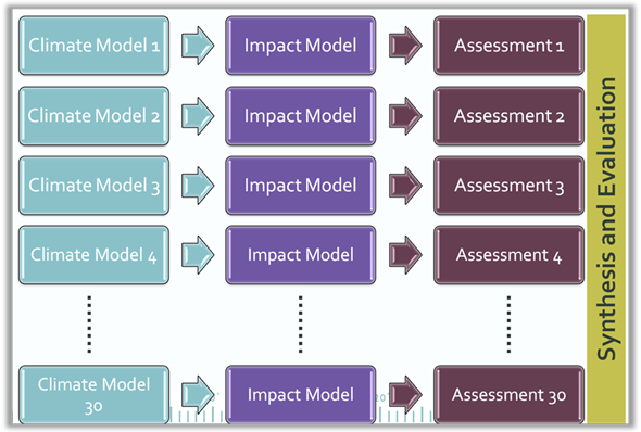
Illustration showing a process of completing the impact assessment using results from many individual climate models followed by synthesis and evaluation of the results.

Figure 1: Conceptual approach to using all available models to undertake a climate change impact assessment with internally consistent data.

A common approach to dealing with this issue has been to select a small number of ‘best’ climate models based on their ability to represent the current climate. This approach suffers from a lack of agreement among climate scientists on how to determine which are the ‘best’ models. Often, a model that performs well in one aspect shows less skill when evaluated for another. Furthermore, this approach does not account for the need to represent the range of uncertainty among the full suite of available model projections.

The characteristics of climate projections for use in impact assessments can be summarised as:

Internally consistent: the projected changes for each of the climate variables are internally consistent.

Adequate sample: the model results used adequately sample the range of the projected changes in a way that is relevant to the impact assessment.

Achievable: the end user has adequate skills and resources to successfully use the amount of data produced.

Inform likelihood assessments: the projections are associated with information on the degree of model agreement that can inform risk assessments for each set of impacts.

The Climate Futures framework has been developed by CSIRO to provide a mechanism for meet these requirements. It does this by classifying the projected changes from all available climate models (for a given emissions scenario and future time period) into categories defined by two climate variables (usually the change in annual mean temperature and rainfall – see Figure 1). Thus, models can be sorted into different categories or ‘Climate Futures’, such as ‘Warmer – Drier’ or ‘Hotter – Much Drier’. A simple table shows the spread in the model results and allows users to explore how this changes under different emissions scenarios and time periods.

The table also shows the amount of agreement among the models (‘model consensus’) for each Climate Future. For example, if 14 of 28 models fall into the ‘Warmer – Drier’ climate future, it is given a consensus score of 50%, described as ‘Moderate Consensus’. Understanding the degree of model consensus for each climate future can help decision makers estimate the likelihoods of particular impacts.

Illustration of the climate futures matrix showing groupings of climate model results.

Figure 2: Example Climate Futures Matrix showing a hypothetical ‘Best’ case (green), ‘Worst’ case (red) and ‘Maximum Consensus’ case (black).

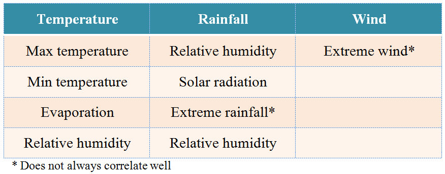
Frequently, an impact assessment will require more than two variables. For example, to evaluate the impact of climate change on sugar cane crops is likely to require data on temperature, rainfall, solar radiation and evaporation. Fortunately, the projected changes in many variables are related (correlated). For example, changes in evaporation are strongly related (correlated) to changes in temperature. However, wind speed does not correlate well with any other variables. Table 1 shows the main variables available in the climate futures web tool and whether they are correlated with temperature, rainfall or wind speed.

For impact assessments, the Climate Futures framework can provide a pragmatic solution to the issue of dealing with ‘too many models’. A user can easily identify the ‘best case’ and ‘worst case’ Climate Futures in terms of their potential impact. These will sometimes have low consensus scores. A third case is often chosen, representing the ‘maximum consensus’ climate future. Thus, for a given emissions scenario and future time period, the user need only undertake their impact assessment with two or three models, each of which represents a Key Climate Future that is relevant to the impact assessment and has been assigned a consensus score (Figure 3). In this way, the impact assessment takes account of the relevant range of uncertainty in the projections.

Table 1: Quick reference guide to which classifier variables to use to obtain data for more than two variables.

Table showing which of the three variables, temperature, rainfall and wind speed, to use as classifiers to obtain meaningful consensus information for each of the other varibales.

The Pacific Climate Futures Web-tool facilitates the use of the framework at National and Sub-national levels, and provides an objective means for selecting a subset of climate models to represent relevant climate futures. The tool provides projections for up to 19 climate variables, 14 time periods and six emissions scenarios. There are three levels of access to accommodate users with different levels of expertise: Basic, Intermediate and Advanced. The Basic interface, freely available to anyone, provides access to information on the projected changes in annual-average temperature and rainfall. The Intermediate interface is accessible to users who have completed this online training course. The interface is self-guided and allows users to obtain projections datasets for multiple variables in terms of the Key Climate Futures (i.e. ‘best’, ‘worst’ and ‘maximum consensus’ cases). The Advanced interface is only available to users who have completed a comprehensive, face-to-face training programme. The Advanced interface is most likely to be of use to researchers.

Illustration showing the simplified process of completing the impact assessment using results from three representative climate models followed by synthesis and evaluation of the results.

Figure 3: Conceptual approach to including climate change information in an impact assessment process using the ‘key climate futures’ approach. Non-climatic factors would be incorporated at the ‘Assessment’ stage.

For some risk assessments, the direction and magnitude of projected change in climate at monthly, seasonal or annual scales averaged over a region of interest is sufficient. These data can be displayed and results from the selected GCMs can be exported from Australian Climate Futures. Many assessments, however, require future datasets that have the characteristics of actual weather, such as a daily time series of maximum temperature and rainfall. Whilst data of this type may be available from a range of methods, it is often sufficient to simply modify a dataset of actual observations (say, from a national meteorological service weather station) with the amounts of change projected by the selected set of GCMs. The Pacific Climate Futures web-tool assists users to do this by exporting the projected changes into a preformatted MS Excel spreadsheet. Users can enter observed data into the spreadsheet which then automatically calculates the plausible future values.

Introduction to Pacific Climate Futures

Climate Projections for Impact Assessment

Further Reading