Introduction to Climate Change Projections

The climate of the Pacific is changing and will continue to change into the future. We will need to plan for these changes and adapt to these changes. To do this, we will need to know what aspects of the climate are going to change, when they are going to change and by how much they are going to change. There are many different people who use climate change information – teachers at schools, policy officers in climate change departments and farmers. Not everyone will need detailed climate projections but it is important to understand the basic concepts of how projections are made.

The climate system is very complex, so you can’t just look at past trends and expect them to continue into the future. For instance, a twenty year increasing trend in rainfall over an oceanic region may cause a change to the local ocean circulation, due to a freshening of the surface waters. This new circulation may transport warm water away from the region, thus inhibiting rainfall and reversing the initial trend.

Instead, a three-dimensional computer representation of the Earth’s climate system known as a Global Climate Model is used to simulate the fundamental processes driving weather and climate. Climate models are mathematical representations of the climate system that require very powerful computers. They are based on the laws of physics which will continue to apply in a changed environment and include information about the atmosphere, ocean, land and ice.

In a Global Climate Model the globe is broken up into lots of little boxes. For the atmosphere, these boxes are typically about 100-400km by 100-400km in the horizontal and there are about 40 layers of them between the surface and the top of the atmosphere.

The model then calculates climate variables such as temperature, rainfall and wind at each of the boxes from mathematical rules based on the laws of physics, such as conservation of mass, energy and momentum. The picture in Figure 1 shows the earth divided up into lots of grid boxes and the breakout square shows the physical processes included in each box – such as solar radiation and ocean currents.

Figure 1: Representation of a global climate model showing the arrangement of grid boxes and processes calculated. (Source: Centre for Multiscale Modelling of Atmospheric Processes)

Global climate models have improved greatly over the past 40 years and continue to improve. The first climate models in the 1970s and 1980s included only rain, sun and carbon dioxide emissions. As models became more complex, volcanic activity, the oceans and clouds were included. The latest climate models (Figure 2) can simulate the changes that occur in vegetation in response to changes in the soil and atmosphere, the complex chemical interactions in the atmosphere, the dynamics of ice sheets and the processes of marine ecosystems.

Figure 2: The components of modern global climate models. (Source: SciDAC Review 2013)

There have also been huge improvements in the resolution of climate models – this means how big each grid box is. The smaller the boxes, the more computer power is needed to run the models. Figure 3 shows past, present and future resolutions. In the earliest climate models (T45), the grid boxes were around 500km. As computers have become more powerful, the boxes have become smaller and the models can produce more detail. Even higher resolution models will become available in future.

Figure 3: Early climate model resolution was around 500 km (T42). Current global climate models have resolutions of around 100 – 150 km (T85). In future, higher resolution (T170, T340) global climate models will become possible as the power of super-computers continues to increase. (Source: UCAR)

There are many research institutions around the world, including Australia’s CSIRO and Bureau of Meteorology, that develop and maintain their own global climate models. There are more than 40 models in the current generation (CMIP5) of global climate models. While these models all apply the same laws of physics, subtle differences exist with respect to factors such as: grid characteristics – e.g. resolution; model sub-components – e.g. not all models have a sea ice component; and parameterisation schemes – the way models estimate factors that operate at scales smaller than their grid box size (for example cloud droplets). These differences among the models mean that the model results are different too.

Global climate models have shown us that most of the global warming since the mid-20^th century is extremely likely due to human activities. Figure 4 shows changes in global average temperatures since 1860. The black lines show the trend based on observations (reconstructed using three different methods). The graph in (a) compares the simulations from the models based on natural factors AND human-induced factors (often called anthropogenic), that is changes in the sun’s radiation, volcanic eruptions as well as changes due to increased greenhouse gases resulting from human activities. Graph (b) compares the observations to only natural factors (e.g. changes in the sun’s radiation and volcanic eruptions) and graph (c) shows only human-induced factors. These graphs show clearly that natural factors alone cannot explain the observed temperature changes since 1860.

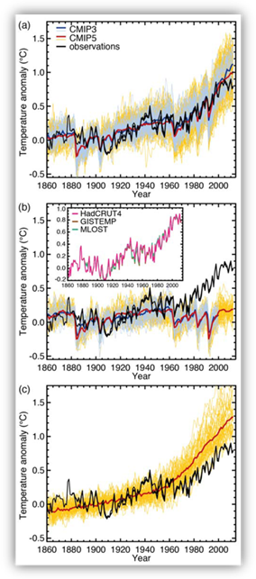
Figure 4: The observed global temperatures (black lines) compared to the corresponding global climate model results from CMIP3 (dark and light blue lines) and CMIP5 (orange and red lines) using natural greenhouse gas inputs only (a), both natural and human-induced greenhouse gas inputs (b), and only human-induced greenhouse gas inputs (c). The combined effect of natural and human-induced greenhouse gas inputs is required to adequately explain the changes in global temperature that have been observed. (Source: IPCC 5^th Assessment Report)

The Intergovernmental Panel on Climate Change, a scientific organisation who reviews and assess the latest scientific, technical and socio-economic climate change information, concluded that most of the global warming since the mid 20^th century is extremely likely due to human greenhouse gas emissions. As we do not know what the future holds, we need to consider a range of possible future conditions, or scenarios. And we use climate models to make projections.

Models are carefully tested. Scientists test the model results against what we know happened in the past and what is currently happening to see if the model can match reality.

The chart in Figure 5 compares the observed global mean surface temperature over the 20^th century (black line) with simulations from 14 global climate models (yellow band).  The red line shows the mean of the models. Vertical grey lines indicate the timing of major volcanic eruptions (which cool the earth).  It can be seen that there is general agreement between the observations (black line) and the model simulations (yellow band).  This shows that the models do a good job at simulating what actually happened to the climate in the past. This is good because it means that they get the basic climate characteristics right and so should be able to produce projections for the future too.

Figure 5: Example of the type of trend assessment undertaken as part of model evaluation. (Source: IPCC AR4)

Due to their limited resolution (the big size of the grid boxes), global climate models can only give you information about the large-scale climate. For example, Figure 6 shows a Global Climate Model simulation (left) of the annual average rainfall total in Tasmania (Australia). It picks up the large scale information, which is essentially that Tasmania is a relatively dry place. However we can see from an image of the actual climate (right) that due to the limited resolution of the model, it fails to recognise the mountain range in the middle of the state, which causes quite high rainfall on the west coast. In other words, the global climate model can’t pick up some of the small scale details.

Figure 6: Historic annual average rainfall over Tasmania (Australia) as simulated by a global climate model compared to the actual rainfall for the same period.

This is an important point to consider when interpreting climate projections coming from global climate models – they only tell you how the large scale climate may change. If a global climate model says it’s going to be wetter over your country, it means that it will generally be wetter in your region of the Pacific, but localised (or small scale) weather effects (such as a mountain range) will mean that it might not get wetter at every location within your country.

We can see from the map in Figure 7 that the models do a good job at simulating the large scale features of the climate. The figure at the top shows the annual average temperature for the period 1980 – 99 as indicated by observations. The figure at the bottom shows that the average of the climate models depicts a very similar result.

Figure 7: Comparison of global climate models simulations with observations for global patterns of temperature

Similarly, the climate model average for the annual average rainfall for the period 1980 – 99 shows strong agreement with the observations (Figure 8).

Figure 8: Comparison of global climate models simulations with observations for global patterns of rainfall.

If we zoom in on the Pacific region, however, the models struggle with some of the precise details of these climate features. Figure 9 shows the annual average rainfall over the 20 year period 1980-1999. On top is the actual (or observed) average rainfall for that period (from a dataset known as CMAP) and on the bottom is the rainfall from the 24 model ensemble (in other words, it is the average of all 24 models). Blue colours indicate high rainfall and brown colours indicate low rainfall.

Figure 9: Rainfall patterns at regional scale showing shortcomings of the models.

The main large-scale features of the rainfall in the Pacific region, including the high rainfall areas associated with the Intertropical Convergence Zone, the South Pacific Convergence Zone and the West Pacific Monsoon, are clearly present in most model simulations.

 
The models do a good job of showing the seasonal reversal of wind-direction over the region to the north of Australia, extending from East Timor to the Solomon Islands and do a good job at representing the rainfall amount. We know that the intensity of the West Pacific Monsoon is associated with ENSO (La Niña = strong monsoon), but some models do really poorly at showing this relationship.
 
The models tend to get the Intertropical Convergence Zone in the right position for February but it moves too far north during July – September. Some models have a split in their ITCZ – creating a double ITCZ.
 
The models do a fairly good job at capturing the changes to the South Pacific Convergence Zone zone during La Niña and El Niño, but overall they show the SPCZ as too zonal (or east-west oriented).

So from looking at this, we can see that when interpreting climate projections, it is important to know about any issues that the models might have with the precise details of the large-scale climate. The Pacific Climate Change Science Program (PCCSP) and the follow-up Pacific-Australia Climate Change Science and Adaptation Planning (PACCSAP) program conducted rigorous evaluations of the global climate models that were available at the time looking at various variables and climate features. From this evaluation, they found there is no single best model. All models have their strengths and weaknesses. However, there were some models that performed consistently poorly across many aspects of climate, so they were excluded when making projections.

Projections are created around future scenarios that have been developed by the Intergovernmental Panel on Climate Change. In their 2007 report their global projections were based on six groups of possible future scenarios. In the 2013 projections they used four different scenarios called Representative Concentration Pathways. Both sets of emissions scenarios are representations of a possible future based on differing sets of assumptions about population changes, economic development and technological advances.  These greenhouse gas emissions scenarios are used in climate modelling to provide projections that represent a range of possible futures. Uncertainty exists around climate projections because we do not know what actions will be taken to mitigate emissions.

Figure 10: Four RCPs describe plausible trajectories of future greenhouse-gas and aerosol concentrations to the year 2100 (solid lines). The earlier SRES scenarios are shown with dashed lines.

When developing climate projections you also need to consider time periods. When we are talking about future projections for a particular year (like 2055), we are not talking about a single year, but the climate averaged over a number of years (e.g. 2045 – 2064) for which 2055 happens to be the central year. Projections relate to the mean climate and should not be confused with a forecast for any particular year.

Projections can be made for a number of different climate variables. The PCCSP and PACCSAP program developed projections for all partner countries for:

• Air temperature (mean, maximum and minimum)
• Rainfall (mean and heavy rainfall)
• Evaporation
• Wind speed (mean and strong wind)
• Relative humidity
• Solar radiation
• Sea surface temperature
• Ocean acidification
• Sea level
• Tropical cyclones

The results of these projections can be found in the web-tool Pacific Climate Futures as well as on the Pacific Climate Change Science website. Your national meteorological service will also be able to provide you with detailed projections for these variables.

Global Climate Models enable us make climate projections for the future, however there is still a large amount of uncertainty about these projections for a number of reasons.

1. Emission scenario uncertainty: We don’t yet know what the emissions scenario for the future will be as we don’t know what mitigation measures will be taken at international and national levels over the next century.
2. Model uncertainty: The PCCSP used 18 models to create projections for the Pacific and they all produce different values for different variables. All models are different and therefore simulate slightly different futures
3. Model skill: Global Climate Models are only giving you information about the large-scale climate and they have some issues with the precise details of that large-scale climate.

A key point to remember when looking at projections is that they are for an average change over a broad geographic region encompassing the country of interest (not a village or city).

Another area to consider when looking at climate projections is natural variability (see Introduction to Climate Variability and Change). As the climate changes, there will continue to be natural variability. So while temperature, for example, will increase on average, there will still be those days which are cool and those days which are warm. However, overall, the climate will be getting warmer. The actual weather in 2055 or 2090 might differ from the projected change in the average climate, due to natural variability (i.e. these are projections of the average climate, not weather forecasts). The graph in Figure 11 shows the range of climate variability that can occur around an increasing trend.

Figure 11: Illustration of how climate change and climate variability occur together.

It is important to understand that there is uncertainty in projections and that scientists have different levels of confidence for different projections. For example, we learnt earlier that due to the large range of natural variability in rainfall it is more difficult to identify climate change trends for rainfall than temperature – similarly there is generally a lower confidence in rainfall projections than in projections of temperature. Scientists in the PCCSP and PACCSAP program used their expert judgment to assign confidence levels to the projections found in the reports. They looked at how much agreement there was between the model simulations, how good the models were at simulating the current climate (particularly for that variable) and how physically plausible the projection was. You can see in the diagram that they used these criteria to assign confidence levels ranging from very low to very high.

Figure 12: Confidence scale and criteria used for the climate projections provided by the PCCSP and PACCSAP.

Climate projections can be obtained from the PCCSP and PACCSAP reports (available from www.pacificclimatechangescience.org) as well as the Pacific Climate Futures web-tool. More detail about the tool is provided in Introduction to Pacific Climate Futures.

In summary

We have learnt that climate projections are important for future planning and for adapting to climate change. The climate system is very complex and so we cannot just look at past trends and say they will continue into the future. Instead we use global climate models to project the future climate. These models can capture the major large-scale features of the Pacific climate very well, but they have problems with some of the precise details.

Next Topic (Introduction to Pacific Climate Futures)